4 Tips to Extract Text and Numbers from a String in Excel You Might Not Know

In this article, I will guide you through 4 tips to extract text and numbers from a string in Excel that you may encounter frequently in your daily life. Let’s explore them below!
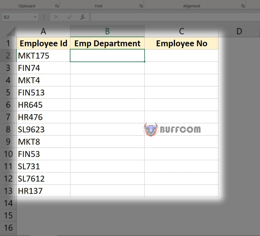
Example: I have a data table like the one below:
4 Tips to Extract Text and Numbers from a String in Excel
Requirement: Based on the data in the Employee Id column, you will extract the strings into 2 parts: extract the employee department code into the Emp Department column and extract the employee number into the Emloyee No column.
To do this, I will use 4 data extraction tips as follows:
Tip 1: Extract text and numbers using Flash Fill
Starting from version 2013, Excel has a very useful new tool called Flash Fill. This is a feature that helps users automatically fill in values, saving time and minimizing the need for unnecessary functions.
To use this tool, follow these steps:
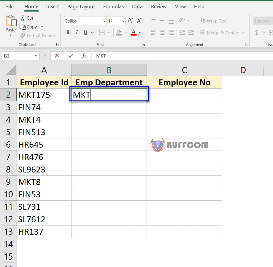
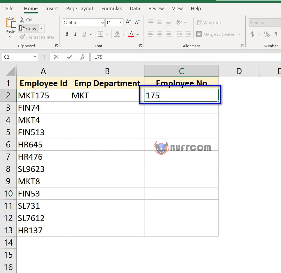
Step 1: In the Emp Department column, at the first cell, type in the department code of the first employee.
4 Tips to Extract Text and Numbers from a String in Excel
Similarly, in the Emloyee No column, type in the number of employees based on the first cell in the Employee ID column.
4 Tips to Extract Text and Numbers from a String in Excel
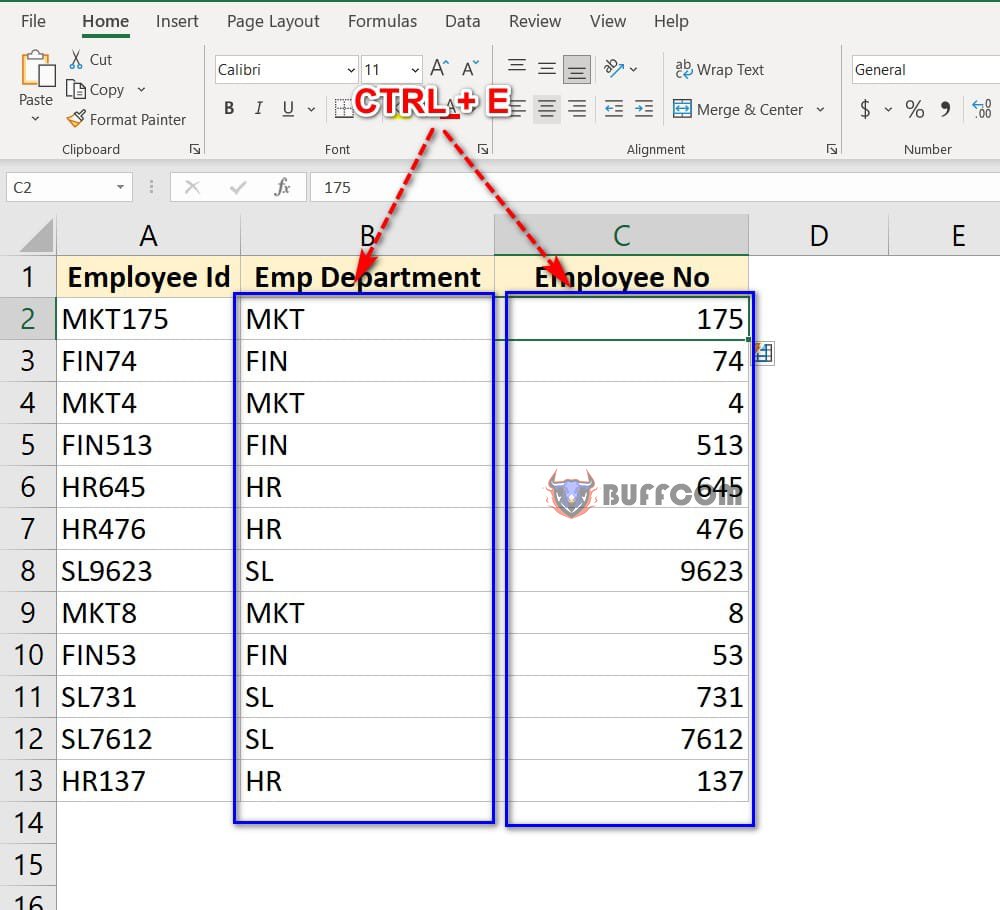
Step 2: At the first cell displaying the first result in the Emp Department column, press Ctrl + E to display the result in the following cells.
Similarly, at the first cell in the Emloyee No column, press Ctrl + E to display the result in the following cells.
4 Tips to Extract Text and Numbers from a String in Excel
Tip 2: Separate letters and numbers using a formula
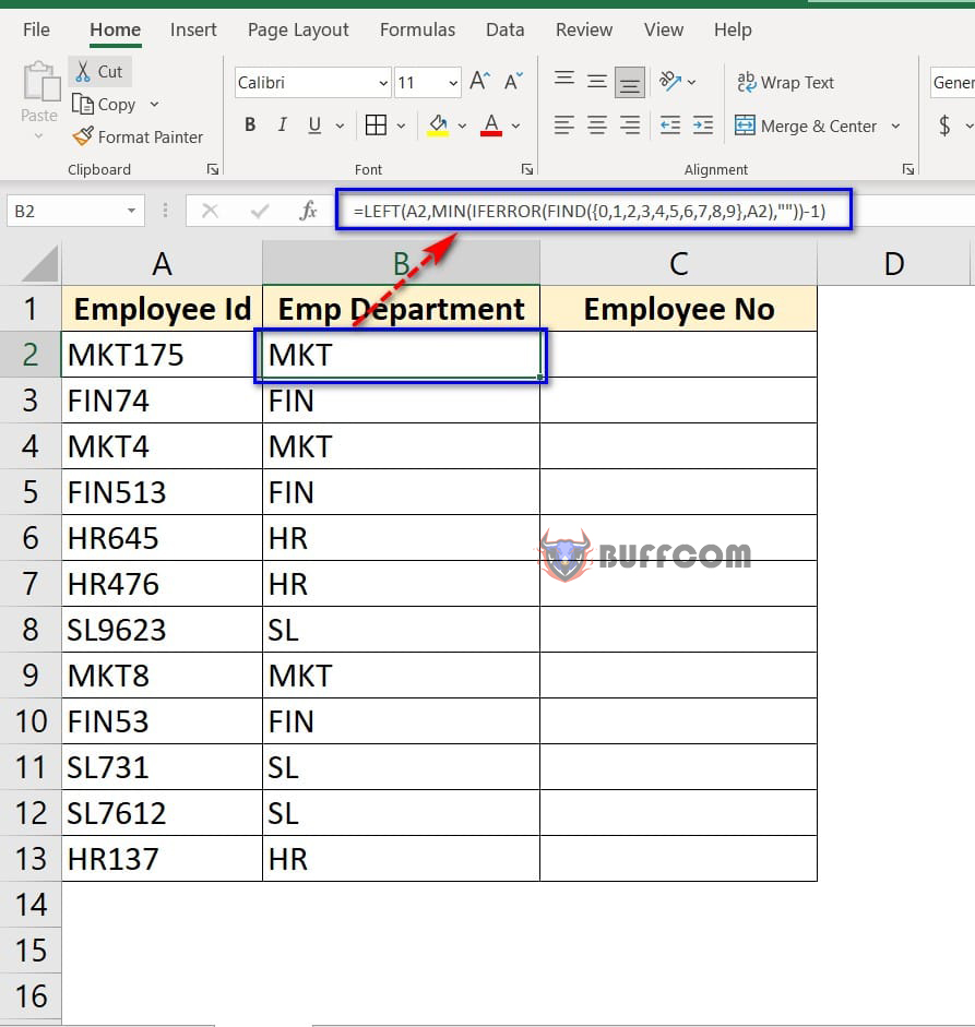
To use this method, in the first cell of the Emp Department column, type the following formula: =LEFT(A2,MIN(IFERROR(FIND({0,1,2,3,4,5,6,7,8,9},A2),””))-1)
Explanation:
4 Tips to Extract Text and Numbers from a String in Excel
Find: Use this function to find the position of numbers from 0 to 9.
A2: The cell that contains the first ID to extract the employee department code.
IFERROR: Use this function to handle cases where no numbers are found or if an error occurs by displaying a blank “”.
Min: Because when using the FIND function, all positions that contain numbers will be displayed. However, we only want to take the position of the first number, so we use the MIN function to get the smallest position number.
LEFT: Use this function to extract the employee department code from the ID cell.
Finally, subtract 1 to only count the number of characters in the employee department code before the numbers in the data.
Similarly, to extract the number of employees into the Employee No column, type: =MID(A2,MIN(IFERROR(FIND({0,1,2,3,4,5,6,7,8,9},A2),””)),100)
Explanation:
Find: Use this function to find the position of numbers from 0 to 9.
A2: The cell that contains the first ID to extract the number of employees.
IFERROR: Use this function to handle cases where no numbers are found or if an error occurs by displaying a blank “”.
Min: Because when using the FIND function, all positions that contain numbers will be displayed. However, we only want to take the position of the first number, so we use the MIN function to get the smallest position number.
MID: Use this function to extract the number of employees from the ID cell.
100: Use the value 100 to estimate the number of characters after the position of the first number.
Tip 3: Separate letters and numbers using VBA
To use this method, first access the VBA interface by:
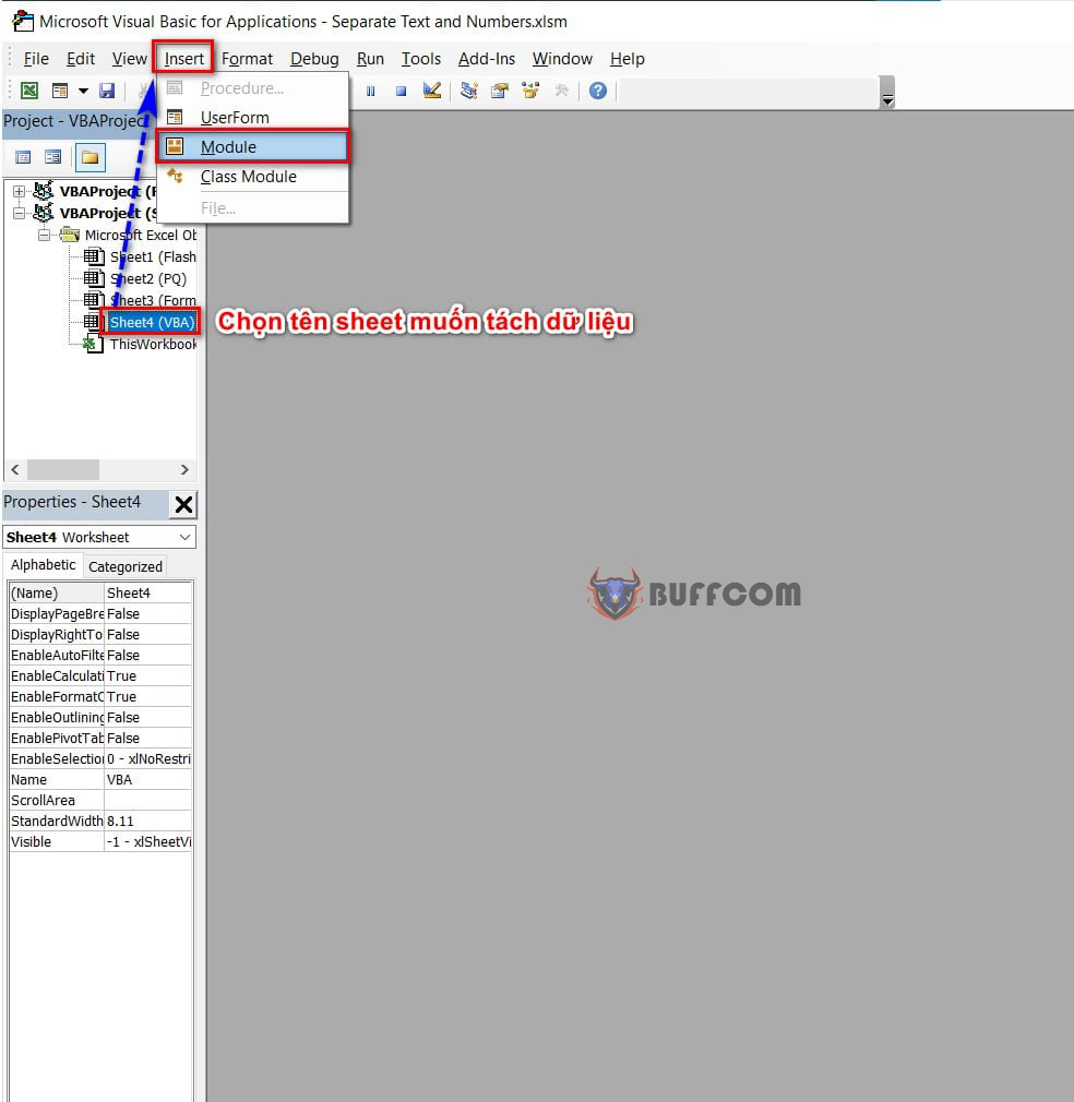
On the worksheet containing the data to be separated, press the key combination ALT + F11.
The VBA interface will appear. Next, you will create a module to contain the code for separating the data by clicking on the Insert tab => selecting Module.
4 Tips to Extract Text and Numbers from a String in Excel
Display the module interface, where you enter the following code:
Function GetNumber(CellRef As String)
Dim StringLength As Integer
StringLength = Len(CellRef)
For i = 1 To StringLength
If IsNumeric(Mid(CellRef, i, 1)) Then Result = Result & Mid(CellRef, i, 1)
Next i
GetNumber = Result
End Function
Function GetText(CellRef As String)
Dim StringLength As Integer
StringLength = Len(CellRef)
For i = 1 To StringLength
If Not (IsNumeric(Mid(CellRef, i, 1))) Then Result = Result & Mid(CellRef, i, 1)
Next i
GetText = Result
End Function
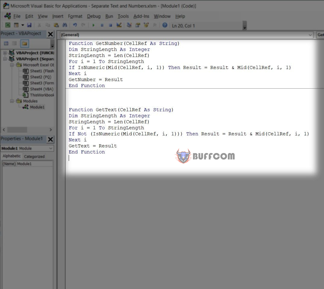
4 Tips to Extract Text and Numbers from a String in Excel
Next, press the Run button on the toolbar or press F5 to run the code.
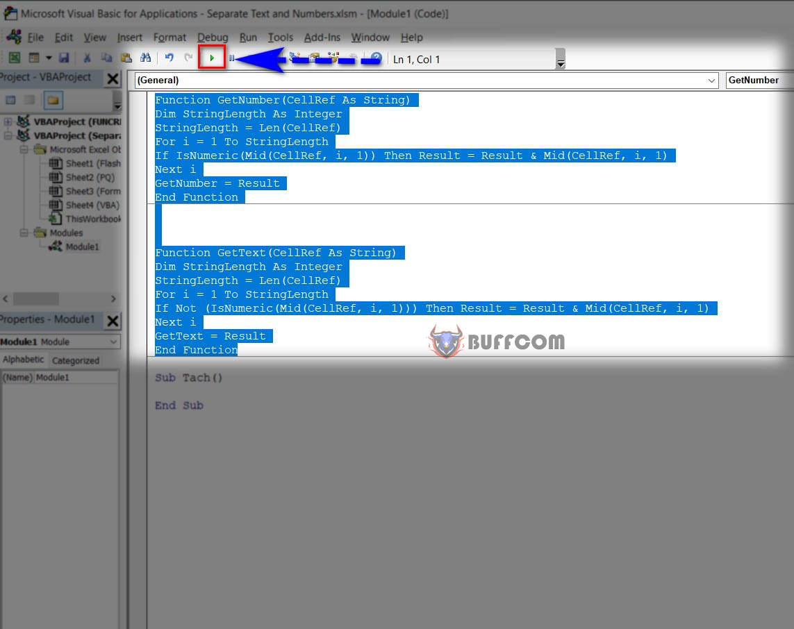
4 Tips to Extract Text and Numbers from a String in Excel
After running, exit the VBA interface.
In the Emp Department column, in the first cell, type: =GetText(A2)
Explanation: The GetText function is created by me from VBA code.
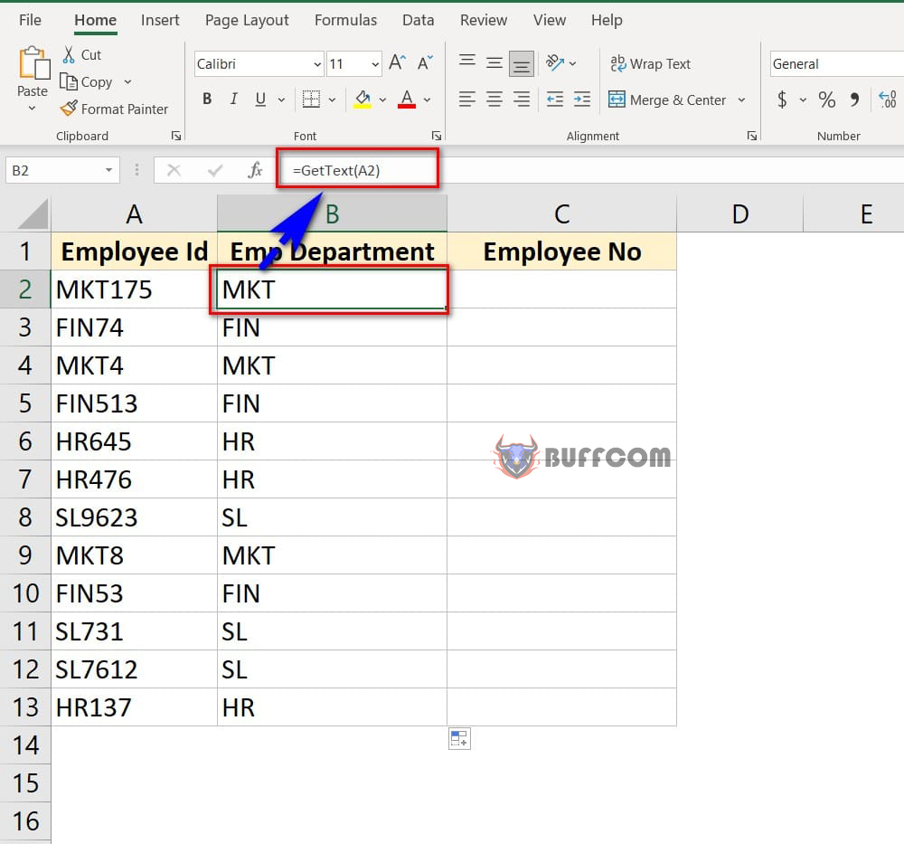
4 Tips to Extract Text and Numbers from a String in Excel
Similarly, to display the Employee No column, in the first cell, type: =GetNumber(A2)
Explanation: The GetNumber function is created by me from VBA code.
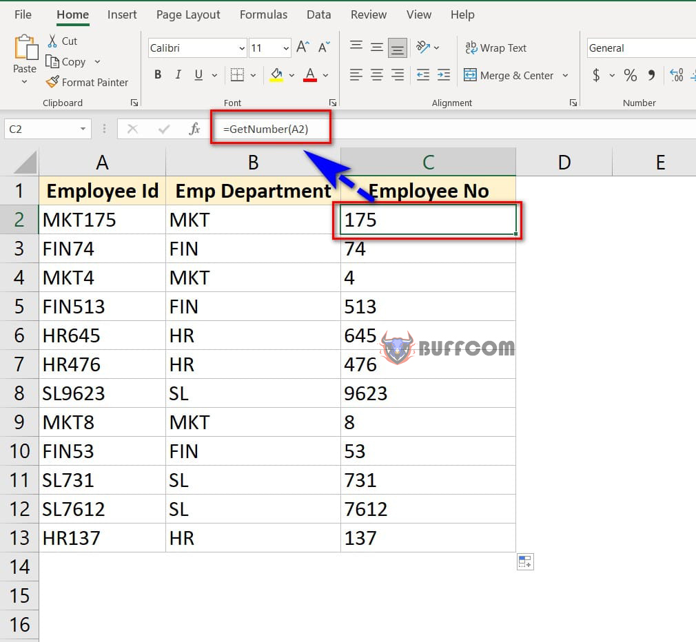
4 Tips to Extract Text and Numbers from a String in Excel
Tip 4: Separating letters and numbers using Power Query
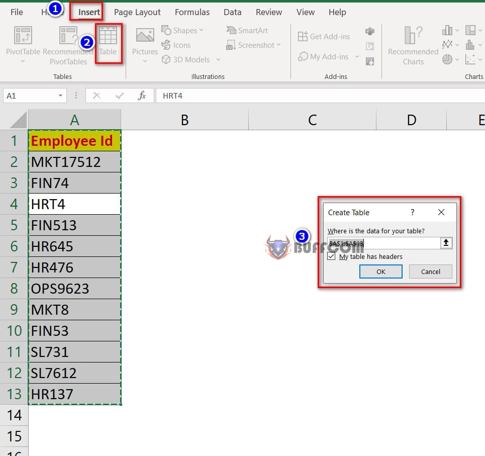
Before using this tip, you need to convert your data into a Table by selecting the data range you want to separate, then go to Insert => Table and press Ok to create the table.
4 Tips to Extract Text and Numbers from a String in Excel
After a table has been created, you can now use the data source query to bring all this data into the query editor. Then, you will separate the text and numbers in the query editor. To do this, go to the Data tab, then select From Table/Range.
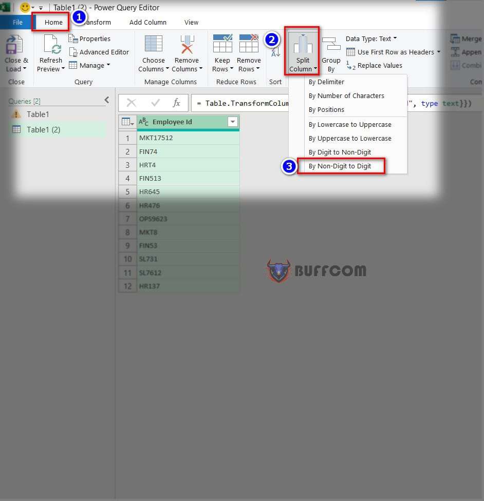
In the Power Query Editor, select the data range you want to separate by clicking on the header. Next, go to Home => Split Column => By non Digit to Digit.
4 Tips to Extract Text and Numbers from a String in Excel
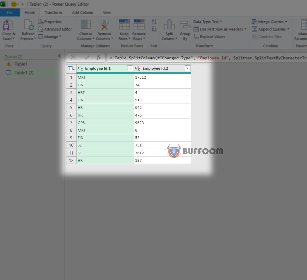
After selecting, your data has been separated.
4 Tips to Extract Text and Numbers from a String in Excel
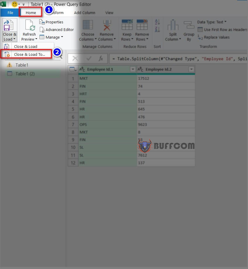
Once completed, you can download the data to an Excel file by going to Home => Close & Load to…
4 Tips to Extract Text and Numbers from a String in Excel
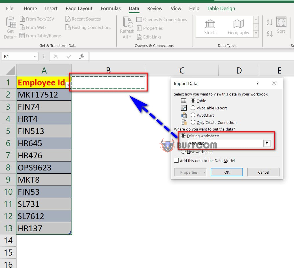
In the Import Data table, select Existing worksheet and choose the location where you want to display the results.
4 Tips to Extract Text and Numbers from a String in Excel
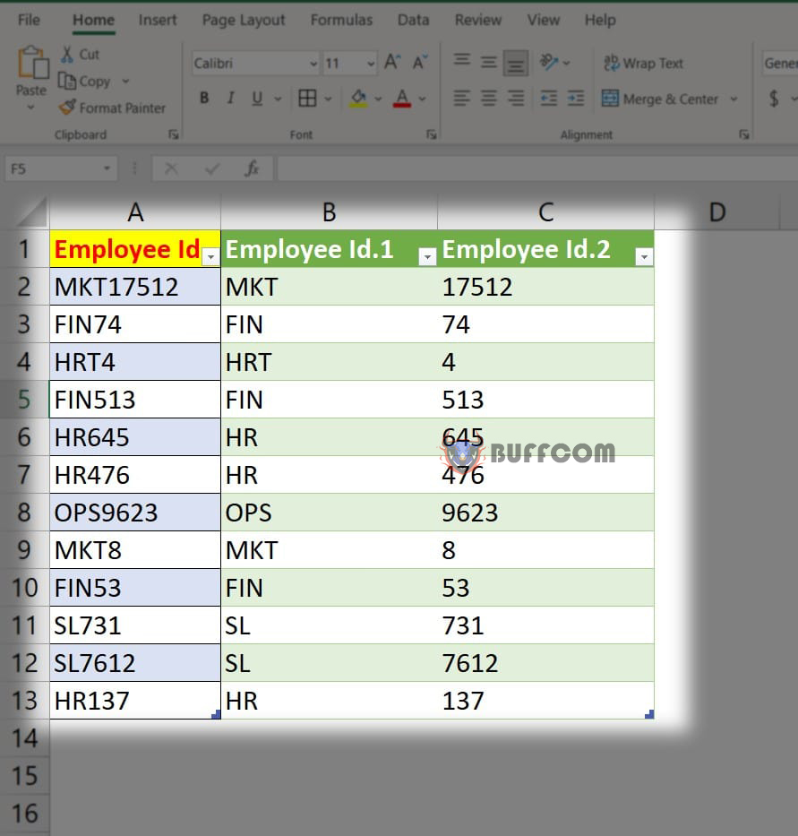
Press OK to complete.
4 Tips to Extract Text and Numbers from a String in Excel
4 Tips to Extract Text and Numbers from a String in Excel
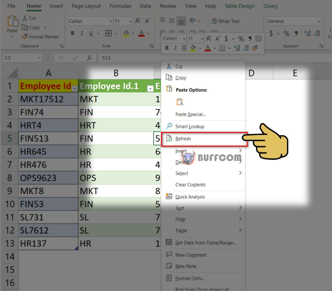
Note: An interesting feature of this tip is that when you edit information in the original data column, the new separated data table will automatically update by selecting any cell in the new data range, right-clicking and selecting Refresh.
So I’ve finished guiding you on 4 tips to separate letters and numbers from strings in Excel that you may not know. Hope this article helps you. If you find it useful, don’t forget to rate the article below! Best regards.

