How to Find the Average of the Highest 5 Values in Excel

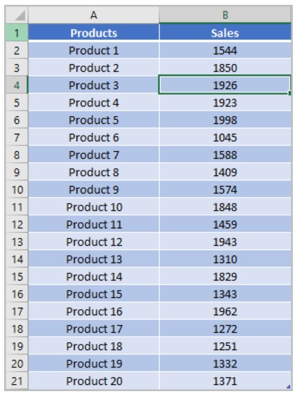
How to Find the Average of the Highest 5 Values in Excel. Suppose you have a list of 20 products in your company and you have monthly sales data for all of them. Now, you want to calculate the average of the top 5 products based on their sales. Here’s an example to illustrate the process.
Formula: Calculate the Average of Top 5 Values
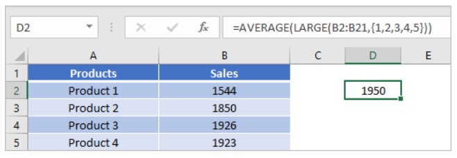
To calculate the average of the top 5 scores from the list, you can use a formula that combines the functions LARGE and AVERAGE. The formula is as follows:
=AVERAGE(LARGE(B2:B21,{1,2,3,4,5}))
Explanation of the Formula
To understand how this formula works, let’s break it down into two parts. In the first part, we use the LARGE function.
LARGE Function
The LARGE function allows you to find the nth largest value in a range of data. If you specify 2 as the nth value, it will return the second-highest value in the data.
In this case, you need the top 5 values, not just one, in order to calculate their average. To achieve this, you need to enter the following array as the nth value:
{1,2,3,4,5}
When you input this array into the function, it returns an array of the top 5 values, similar to the example below:
[1500, 1200, 1000, 900, 800]
Finally, the AVERAGE function calculates the average of these values. It’s important to note that when using an array as an input for the AVERAGE function, you need to enter the formula as an array formula by pressing Ctrl + Shift + Enter.
By following this method, you can easily calculate the average of the top 5 values in Excel.


