How to freeze rows and columns in Excel using Freeze Panes

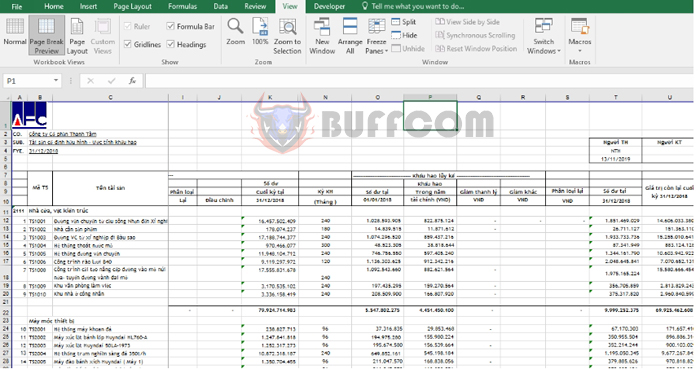
How to freeze rows and columns in Excel using Freeze Panes: Freezing rows and columns allows you to keep track of specific content in long data tables without having to scroll up. Typically, in spreadsheets, we often choose header rows and the content of the first column to freeze, so no matter where we scroll, we can still see which column or row pertains to which content. In addition to freezing a single column or row in Excel, we can also expand to freeze more rows and columns as desired. The following article will guide you on how to use Freeze Panes to freeze columns or header rows.

1. Using Freeze Panes to freeze columns in a worksheet

Freezing the first column of the worksheet
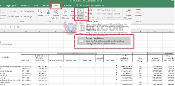
If you only need to freeze the first column of the worksheet, select the View tab => Freeze Panes => Freeze First Column.
This will freeze the first column of the worksheet and keep it visible no matter how far you scroll horizontally.

Freezing multiple columns in the worksheet

If you want to freeze more than one column, place the mouse pointer in the first cell of the next column after the columns you want to freeze (all columns to the left of the cell where you place the pointer will be frozen).
For example, if you want to freeze columns A to C, place the mouse pointer in the first cell of column D, such as D1, as shown below.

Then, select the View tab => Freeze Panes => Freeze Panes.

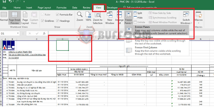This will freeze columns A to C of the worksheet and keep them visible no matter how far you scroll horizontally.

2. Using Freeze Panes to freeze rows in a worksheet

Freezing the first row of the worksheet

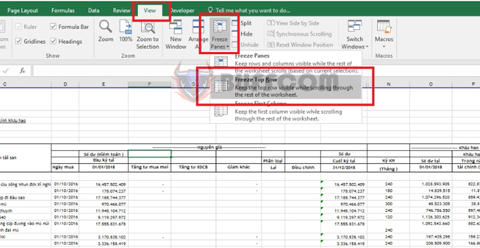
If you need to freeze the first row of the worksheet, select the View tab => Freeze Panes => Freeze Top Row.
This will freeze the first row of the worksheet and keep it visible no matter how far you scroll vertically.

Freezing multiple rows in the worksheet

If you need to freeze more than one row, place the mouse pointer in the first cell of the row below the rows you want to freeze (all rows above the cell where you place the pointer will be frozen).
For example, if you want to freeze rows 1 to 10, place the mouse pointer in the first cell of row 11, which is A11, as shown below.

Then, select the View tab => Freeze Panes => Freeze Panes.

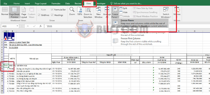This will freeze rows 1 to 10 of the worksheet and keep them visible no matter how far you scroll vertically.

3. Using Freeze Panes to freeze both rows and columns in a worksheet

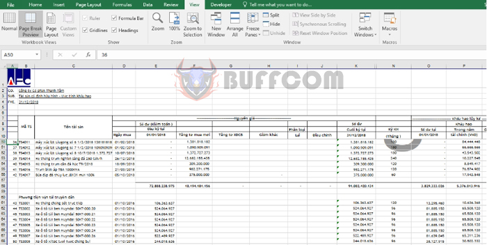
If you want to freeze both rows and columns of the worksheet, you need to determine the position of the mouse pointer. All rows above the row where the pointer is placed will be frozen, and all columns to the left of the column where the pointer is placed will be frozen.
For example, if you want to freeze the first 10 rows and the first 3 columns, place the mouse pointer in the cell at the 4th column of row 11, which is D11, as shown below.

Then, select the View tab => Freeze Panes => Freeze Panes.

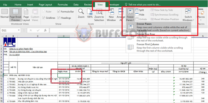This will freeze the first 10 rows and the first 3 columns of the worksheet and keep them visible no matter how far you scroll horizontally or vertically.

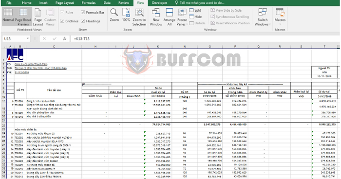4. Unfreezing rows and columns

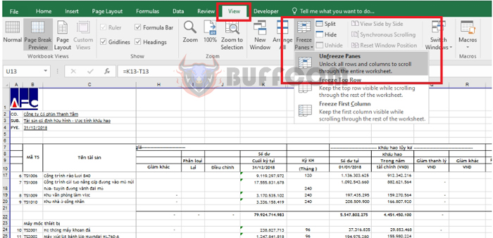
If you no longer want to freeze rows and columns, simply select the View tab => Freeze Panes => Unfreeze Panes.

How to freeze rows and columns in Excel using Freeze Panes

That’s it! The above article has provided guidance on how to freeze rows and columns in a worksheet using Freeze Panes. Good luck with your Excel tasks!