‘Awesome trick’ to insert images into a cell in Excel that is extremely useful

How to insert an image into a cell in Excel so that the image can automatically scale each time the size of the Excel cell changes? In this article, Buffcom.net will guide you on how to insert an image into a cell in Excel.

Microsoft Excel is a powerful spreadsheet software that is widely used around the world with many outstanding features. In this article, Buffcom will delve into how to insert an image into a cell in Excel so that every time you interact with the cell (hide cell, use data filter, move cell to another position, etc.), the image inserted in the cell will also automatically change accordingly.

In the illustration below, the logos of popular companies are placed in the column next to the brand names. Each time you use the filter in the Company name column, the image in the logo column will also be filtered along with the company name data.

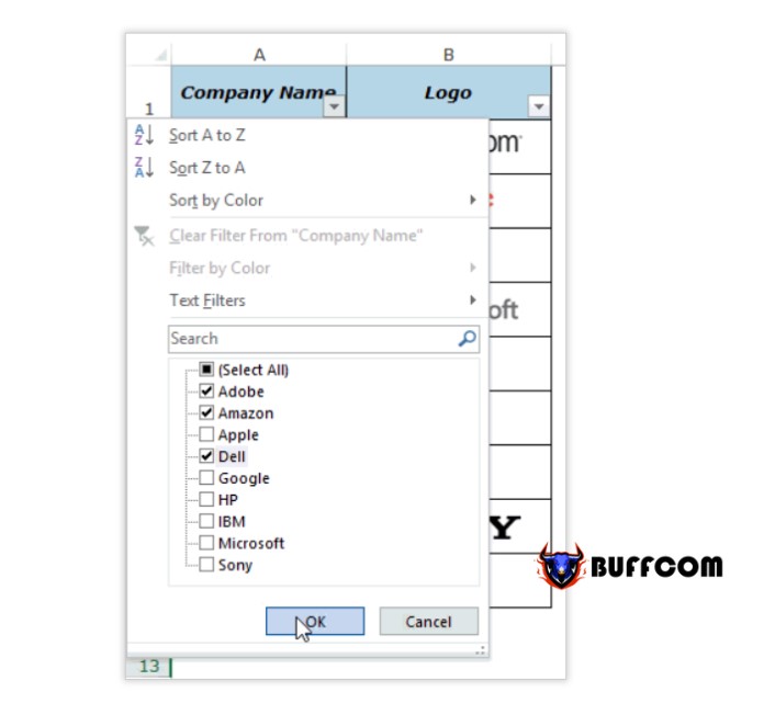This feature is extremely useful if you are doing business and working with many products with corresponding images and product codes.

When you insert an image into a cell in Excel, the image in that cell is not yet linked to other cells and cannot perform operations such as filtering data, moving, hiding, and resizing according to the cell. In the guide below, GhienCongNghe will guide you through each step to insert an image into a cell in Excel as well as to lock the image with the cell in Excel so that every time you interact with the cell (hide cell, use data filter, move cell to another position, etc.), the image will automatically change to fit.

Inserting an image into a cell in Excel

Here is a detailed guide on how to insert an image into a cell in Excel:

1. Open the Insert tab.

2. Click on the Pictures option (under the Illustrations group).

3. The ‘Insert Picture’ dialog box appears, please locate the folder containing the image you want to insert, then highlight to select (you can insert one or multiple images at the same time).

4. Click Insert to insert the image.

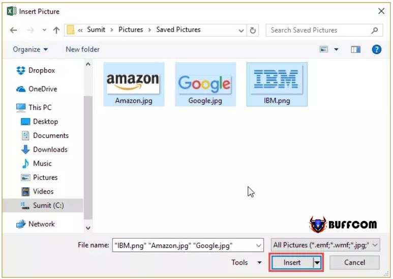5. Resize the image to fit the size of the Excel cell.

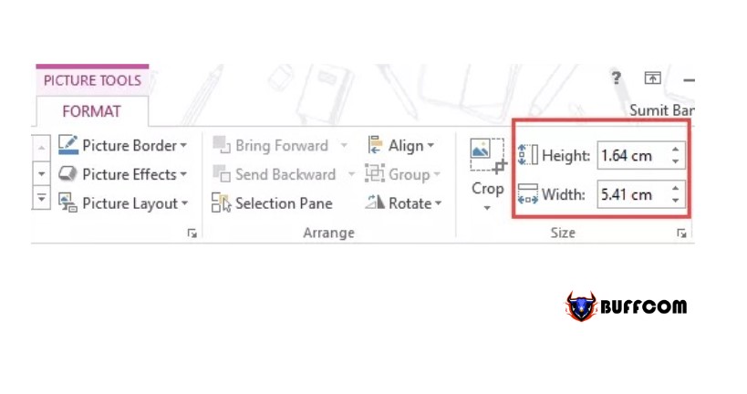6. Insert the image into the cell in Excel.
You can hold down the ALT key and then drag the image to be inserted into the cell by left-clicking and dragging the image to the desired cell. The image will automatically adjust to fit the border of the Excel cell.

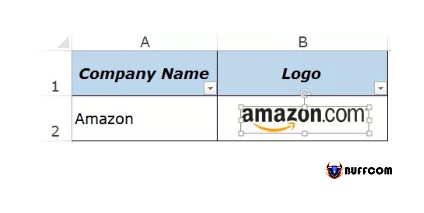If you want to insert multiple images into a cell at once, you can select multiple images at once in step 4 above.

You can also resize the image by selecting it, then dragging the border to adjust the desired size. In case you want to keep the aspect ratio of the logo image, product image, drag the corner of the image to adjust.

Once the image is in the cell after completing the above steps, the image needs to be locked with the cell to be able to resize, use filters, or hide the cell. You need to perform the image lock operation with Excel cell, please follow the instructions below:

Lock the image with the cell in Excel

After inserting the image into the spreadsheet, first resize it to fit in the cell, then follow these steps:
1. Right-click on the image and select Format Picture.

2. In the Format Picture control panel, select Size & Properties (illustrated icon) and then check the ‘Move and size with cells’ option to lock the image to the cell in Excel.

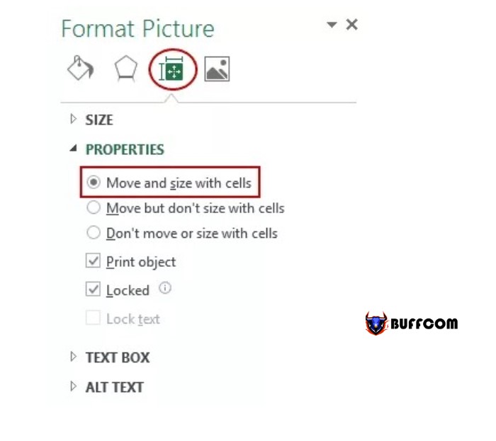So you have completed the task of locking the image into the cell in Excel, every time you interact with the cell with hidden operations, use data filters, move the cell to another position, etc. The image will automatically adjust to fit the cell.

Through this article, Buffcom has presented a tip for inserting an image into a cell in Excel. This tip is really useful in managing lists of items with corresponding images, you can apply it to classify products with images by category, thereby making the work easier and more efficient than ever.

If you find this article useful, please Like & Share to support the team or leave a comment below to discuss if you have a better solution. Thank you for following.