Forecast vs Actual Variance Calculation in Excel

Forecast vs Actual Variance Calculation in Excel. Forecasting plays a crucial role in business management, and comparing actual outcomes with forecasts is essential for project evaluation. To facilitate this process, having a reliable tool or dashboard to calculate the variance between actual and forecasted data is essential. In this article, we will explore how to compare forecasted and actual data in Excel using formulas.

Forecast vs Actual Variance Calculation in Excel

Forecast vs Actual Variance Calculation in Excel

Generic Formula for Variance in Forecast and Actual:

To calculate the variance between forecast and actual data, you can use the following formula:

=ACTUAL – FORECAST

Where: ACTUAL: Represents the actual data or amount obtained. FORECAST: Denotes the forecasted data or amount.

By simply subtracting the forecast from the actual, we expect the actual value to be larger than the forecast. However, if you anticipate the actual value to be less than the forecast, the formula will be reversed.

Forecast vs Actual Variance Calculation in Excel

Let’s proceed with an example to create a Forecast vs Target Report with Variance in Excel:

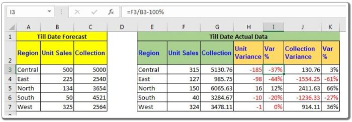
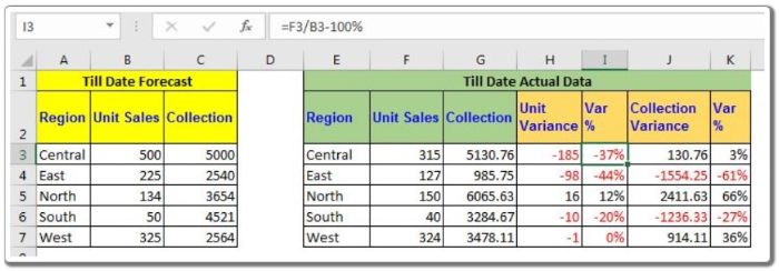
Imagine you have data on the sales of stationery products for different months. By utilizing some Excel forecast formulas, you have generated forecasts for sales and unit production to date. As the months progress, you gather the actual sales and production data in Excel. Now, you want to generate a report that showcases the variance between the actual and forecasted values. Variance, in this context, refers to the difference between the two values. No special variance formula is required; a simple subtraction will suffice.

To calculate the variance between actual and forecasted units, use the following formula in cell H2 and drag it down (for this example):

=F3 – B3

This formula will give you the difference between the Actual and Forecasted unit variance. If the actual value exceeds the forecasted value, you will see a positive difference; otherwise, a negative difference will be displayed.

Similarly, to calculate the variance in collections, write this formula in cell J2 and drag it down:

=G3 – C3

Now, to obtain the percentage variance of units and collections, use these Excel formulas:

=F3 / B3 – 100%

=G3 / C3 – 100%

A negative percentage will indicate a negative variance, while a positive percentage will represent a positive variance. To enhance visibility, you can conditionally format this column to highlight negative values with red text.

Forecast vs Actual Variance Calculation in Excel

In conclusion, creating reports on actual vs. forecasted data using these formulas will facilitate analysis and aid in decision making. I hope the explanation was clear enough. If you have any specific queries regarding forecasting formulas in Excel or any other Excel-related topics, feel free to ask in the comments section below.