Quick tips for calculating table data in Excel
Quick tips for calculating table data in Excel: Excel provides users with many tools to manipulate data in a table. In this article, Buffcom.net will share with you a quick way to calculate data in a table in Excel.
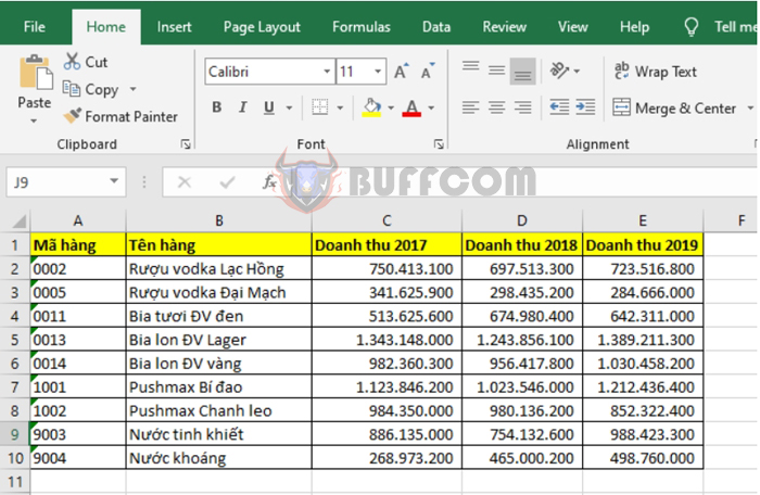
For example, we have a table of revenue for the years 2017, 2018, and 2019 as shown below.
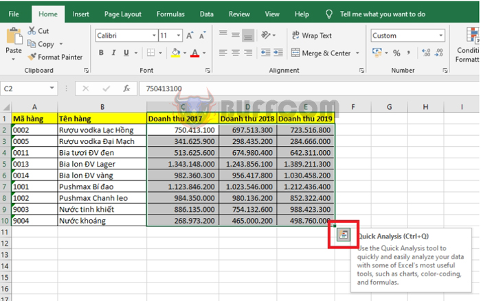
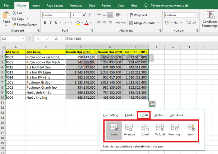
To calculate data in the table, first select all the data cells you want to calculate in the table. Then, click and hold the bottom right corner of the selection. A Quick Analysis tool icon will appear. Click on this icon.
After clicking on the Quick Analysis tool icon, a dialog box will appear. Select the Totals tab. Here you will see calculation functions you can choose from, such as:
Quick tips for calculating table data in Excel
Sum: calculates the sum
Average: calculates the average
Count: counts the number of cells with data
% Total: calculates the percentage of the total
…
Quick tips for calculating table data in Excel
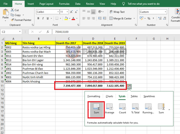
For example, if you want to calculate the total revenue for each year, select the Sum function for each column. The total of each revenue column will be displayed at the bottom of each revenue column in the table.
Quick tips for calculating table data in Excel
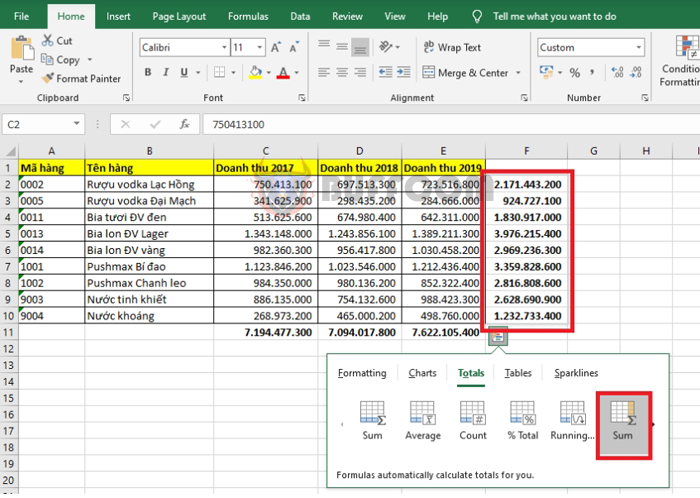
If you want to calculate the total revenue for each product over the 3 years, you can select the Sum function for each row. The total revenue for each product over the 3 years will be displayed to the right of the table.
 In this way, the above article has guided you on how to quickly calculate data in a table in Excel. We hope the article will be useful to you in your work. Good luck!

