• Microsoft Office
  • Microsoft Windows
  • Other Software
  • Anti Virus
  • Blog
    • Word
    • Excel
    • Powerpoint
    • Software tricks/tips
  • POLICIES
    • PAYMENT GUIDE
    • SHIPPING POLICY
    • REFUND POLICY
    • TERMS & CONDITIONS
    • Contact Us

No products in the cart.

  • Microsoft Office
  • Microsoft Windows
  • Other Software
  • Anti Virus
  • Blog
    • Word
    • Excel
    • Powerpoint
    • Software tricks/tips
  • POLICIES
    • PAYMENT GUIDE
    • SHIPPING POLICY
    • REFUND POLICY
    • TERMS & CONDITIONS
    • Contact Us

No products in the cart.

  • Microsoft Office
  • Microsoft Windows
  • Other Software
  • Anti Virus
  • Blog
    • Word
    • Excel
    • Powerpoint
    • Software tricks/tips
  • POLICIES
    • PAYMENT GUIDE
    • SHIPPING POLICY
    • REFUND POLICY
    • TERMS & CONDITIONS
    • Contact Us

No products in the cart.

  • Microsoft Office
  • Microsoft Windows
  • Other Software
  • Anti Virus
  • Blog
    • Word
    • Excel
    • Powerpoint
    • Software tricks/tips
  • POLICIES
    • PAYMENT GUIDE
    • SHIPPING POLICY
    • REFUND POLICY
    • TERMS & CONDITIONS
    • Contact Us
Excel

Highlighting Rows that Meet Criteria in Excel’s Search Box

0 Comments

Highlighting Rows that Meet Criteria in Excel‘s Search Box. This article discusses how to highlight rows in Excel that meet specific criteria in the search box. Previously, we learned how to highlight entire rows if any cell in the row contains specific text. Now, we will focus on highlighting rows if a cell in a particular column contains a specific value. We can achieve this using conditional formatting.Highlighting Rows 1
Highlighting Rows that Meet Criteria in Excel’s Search Box

To highlight rows based on a criteria in Excel, we can use the following generic formula:

= (cell with relative row = criteria)

Here, the “cell with relative row” refers to a cell reference where the column is absolute and the row is relative (e.g., $A1). You can learn more about referencing in Excel here. The “criteria” represents the value or condition that you want to match and highlight the rows.

For example, let’s consider a dataset of fruits. We want to highlight entire rows if the fruit rate is greater than 100. To do this, follow these steps:

  1. Select the first row of the table (e.g., A2:C2).
  2. Go to conditional formatting and choose the “New Rule” option (you can also use the shortcut ALT>H>L>N).
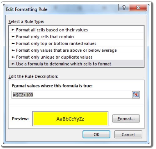
  3. Select “Use a formula to determine which cells to format.”
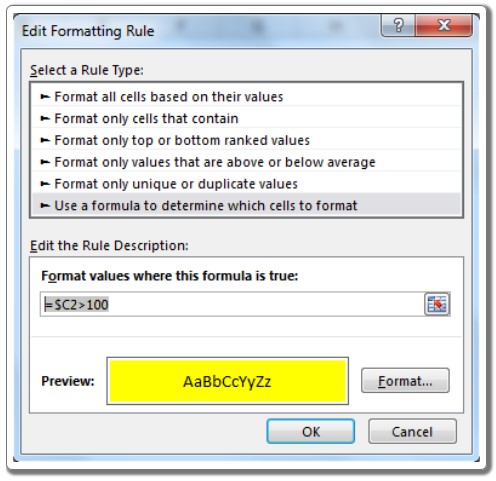
  4. Enter the following formula: =$C2>100Highlighting Rows 2

Note that it is necessary to select the entire row before applying conditional formatting. 5. Click on the “Format” button and choose the fill color (e.g., yellow). Click “OK.”

Now, copy this range and paste the special format to the entire table.Highlighting Rows 3
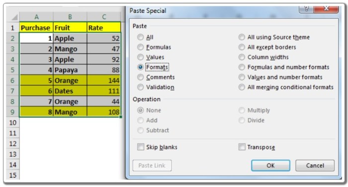
As a result, each row with a rate greater than 100 will be highlighted. In the given example, we hardcoded the criteria, but you can also use cell references.

How does it work? It’s simple. We check if the value in $C2 is greater than 100. If it is, Excel applies the formatting to highlight the entire row. The column reference ($C) is absolute to maintain consistency, while the row reference (2) is relative to adjust accordingly when copying the conditional formatting.

Understanding the concepts of absolute and relative referencing in Excel is key to applying these formatting techniques easily.

We hope this article about highlighting rows that meet criteria in Excel’s search box has been explanatory.

4
36 Views
8 Microsoft Word Tips for Creating Professional-Looking Documents ( P1 )Prev8 Microsoft Word Tips for Creating Professional-Looking Documents ( P1 )July 4, 2023
Compilation Of Useful Keyboard Shortcuts In Windows 10July 5, 2023Compilation Of Useful Keyboard Shortcuts In Windows 10Next

Leave a Reply Cancel reply

Your email address will not be published. Required fields are marked *

Recent Posts
  • Retrieve Data Based on Data Validation
    September 7, 2023
    Excel
  • How to Convert Multiple Rows to Columns and Rows in Excel?
    September 6, 2023
    Excel
  • VLOOKUP for Automatic Discount in Data Validation
    September 6, 2023
    Excel
  • How to Convert Text Dates to Dates in Excel?
    September 5, 2023
    Excel
Categories
  • Blog 80
  • Excel 754
  • Powerpoint 36
  • Software tricks/tips 128
  • Uncategorized 8
  • Word 109
Tags
the ISERROR
Top rated products
  • Kaspersky Small Office Security 15 PCs + 15 Mobiles + 2 Servers 1 Year Kaspersky Small Office Security 15 PCs + 15 Mobiles + 2 Servers 1 Year
    Rated 5.00 out of 5
    $201.00
  • Buy Windows 11 Professional MS Products CD Key
    Rated 5.00 out of 5
    $11.00
  • AVG Internet Security 2021 1 Device 1 Year Global AVG Internet Security 2021 1 Device 1 Year Global
    Rated 5.00 out of 5
    $11.00
  • Buy Office 2021 Professional Plus Key Global For 5 PC
    Rated 5.00 out of 5
    $45.00
  • Avast SecureLine VPN 2021 2 Years 5 Devices Global Avast SecureLine VPN 2021 2 Years 5 Devices Global
    Rated 5.00 out of 5
    $47.00
Products
  • Buy Office 2021 Professional Plus Key Global For 5 PC
    Rated 5.00 out of 5
    $45.00
  • Buy Office 2021 Professional Plus Key Global Bind To Your Microsoft Account
    Rated 4.83 out of 5
    $49.00
  • Windows Server 2022 Datacenter Key Global
    Rated 5.00 out of 5
    $15.00
  • Windows Server 2022 Standard Key Global
    Rated 4.47 out of 5
    $15.00
  • Windows Server 2022 Remote Desktop Services Device Connections (50) Cal Key Global
    Rated 5.00 out of 5
    $45.00

Buffcom.net always brings the best digital products and services to you. Specializing in Office Software and online marketing services

BIG SALE 50% IN MAY

Microsoft Office
Microsoft Windows
Anti-Virus
Contact Us

Visit Us:

125 Division St, New York, NY 10002, USA

Mail Us:

buffcom.net@gmail.com

TERMS & CONDITIONS | PAYMENT GUIDE  | SHIPPING POLICY  | REFUND POLICY

Copyright © 2019 buffcom.net  All Rights Reserved.