Tip on using the LEN function to filter data in Excel

Tip on using the LEN function to filter data in ExcelThe LEN function counts the number of characters in an Excel cell. In this article, Buffcom.net will introduce you to a tip on using the LEN function to filter data in Excel.

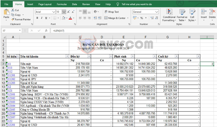
For example, suppose we have a balance sheet as shown in the figure below. The balance sheet is extracted from accounting software and contains many level 1, 2, 3, and 4 accounts. The requirement is to highlight the level 1 accounts for easy identification.

In this case, the LEN function will help us do this very easily. Follow these steps to filter level 1 accounts.

Step 1

First, place the mouse cursor outside the table at the first account. Then use the LEN function to refer to the account using the syntax:

=LEN(A7)

The function will give a result of 3 because the account 111 has 3 characters.

Tip on using the LEN function to filter data in Excel

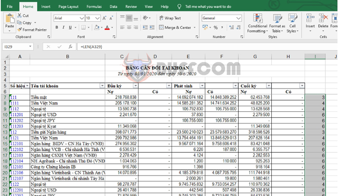
Step 2: Next, copy the above formula to all cells below.

Tip on using the LEN function to filter data in Excel

Step 3

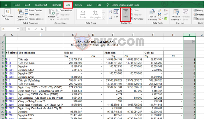
Now, select the entire column I. Then choose the Data tab on the toolbar => select the Filter icon in the Sort & Filter section.

Step 4

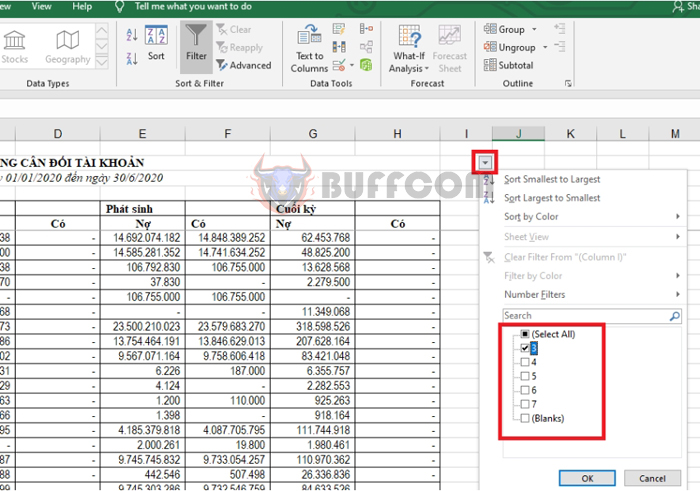
Click on the Filter icon that appears. Then uncheck all items and only select item 3. Then click OK to complete.

Tip on using the LEN function to filter data in Excel

Step 5

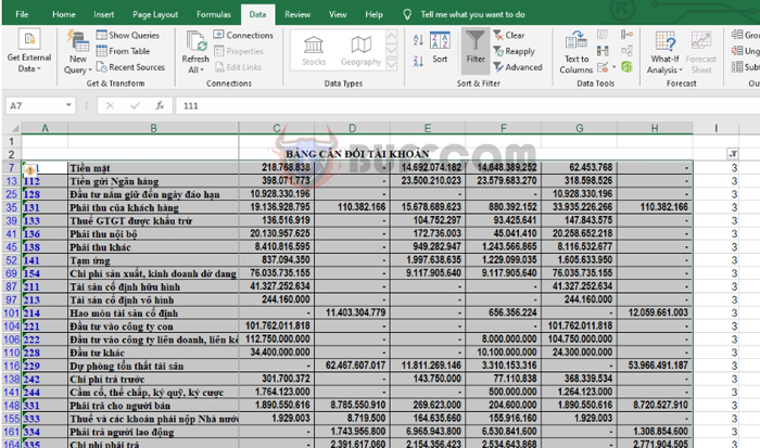
Now, all level 1 accounts with 3 digits are filtered out. You just need to select and highlight them as desired.

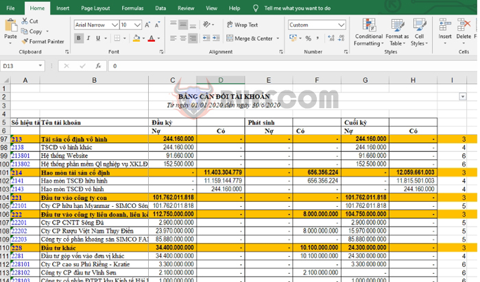
Remove the filter and you have the highlighted balance sheet.

Tip on using the LEN function to filter data in Excel

Thus, the article has instructed you on how to use the LEN function to filter data in Excel. Hopefully, the article will be useful to you in your work. Good luck!